Evolution of the NBA Shot Chart

Evolution of the NBA jump shot heatmap. Demar Derozan must be lonely on the deep-two's islands!

I was sent a link to a GitHub repo containing every shot attempted in the NBA from the 2004 to 2024 season, and felt the gears start turning in my head. With such a rich, dense set of data, there was sure to be some insights to be gained. The data was stored in CSV files, one per season, which made loading, processing, and visualizing the year by year data difficult. Seeking a better approach, I was led to nba-sql, a Python based library that can be used to scrape all sorts of data from stats.nba.com. What was appealing to me about this library was that the data could be stored in an SQLite relational database. In addition to being better equipped to handle and query this large quantity of data, this approach also provided a nice playground to brush up on my SQL and learn about object-relational mapping (ORM). You can read about my ORM journey at the end of the post.

To generate the animation above, I scraped the entire shot chart data base for each year from 1997-98 to 2024-25, which required some minor modifications to the nba-sql library (at first, only the most recent seasons shot chart data was accessible). To isolate jumpers, I filtered out all layups and dunks by removing any attempts in the restricted area. This likely included some non-jump shot attempts, just outside the resricted area (e.g. floaters), but was more reliable than using the shot descriptions included in the dataset (the descriptions included fluctuated dramatically year-to-year). I then generated heatmaps for each year, stitching the results into an animation showing the evoluation over the past ~30 years.

I found the gradual formation of the “deep-two’s” islands interesting. What once were hotspots for shot attemps in the 90’s became nearly compltely removed from the game in the 20’s (save for Demar Derozan, our mid range king). These shots have of course migrated to the three point line, but have also trickled into the paint. We can analyze this more carefully by breaking down the shot attempts by zone.

Jump Shot Attempts by Zone

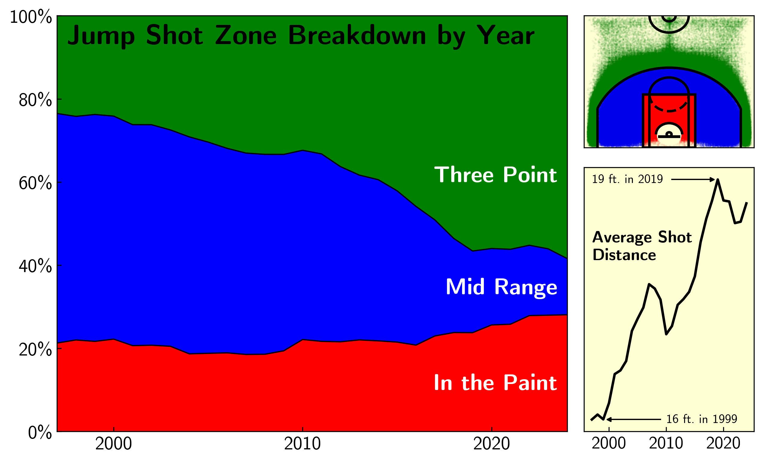
The share of jump shots attempted in the mid range (blue) has shrunk from nearly 55% in 1997 to just 14% in 2024! Meanwhile three attempts (green) have increased from 24% to 58%, and paint shots (red) from 21% to 28%.

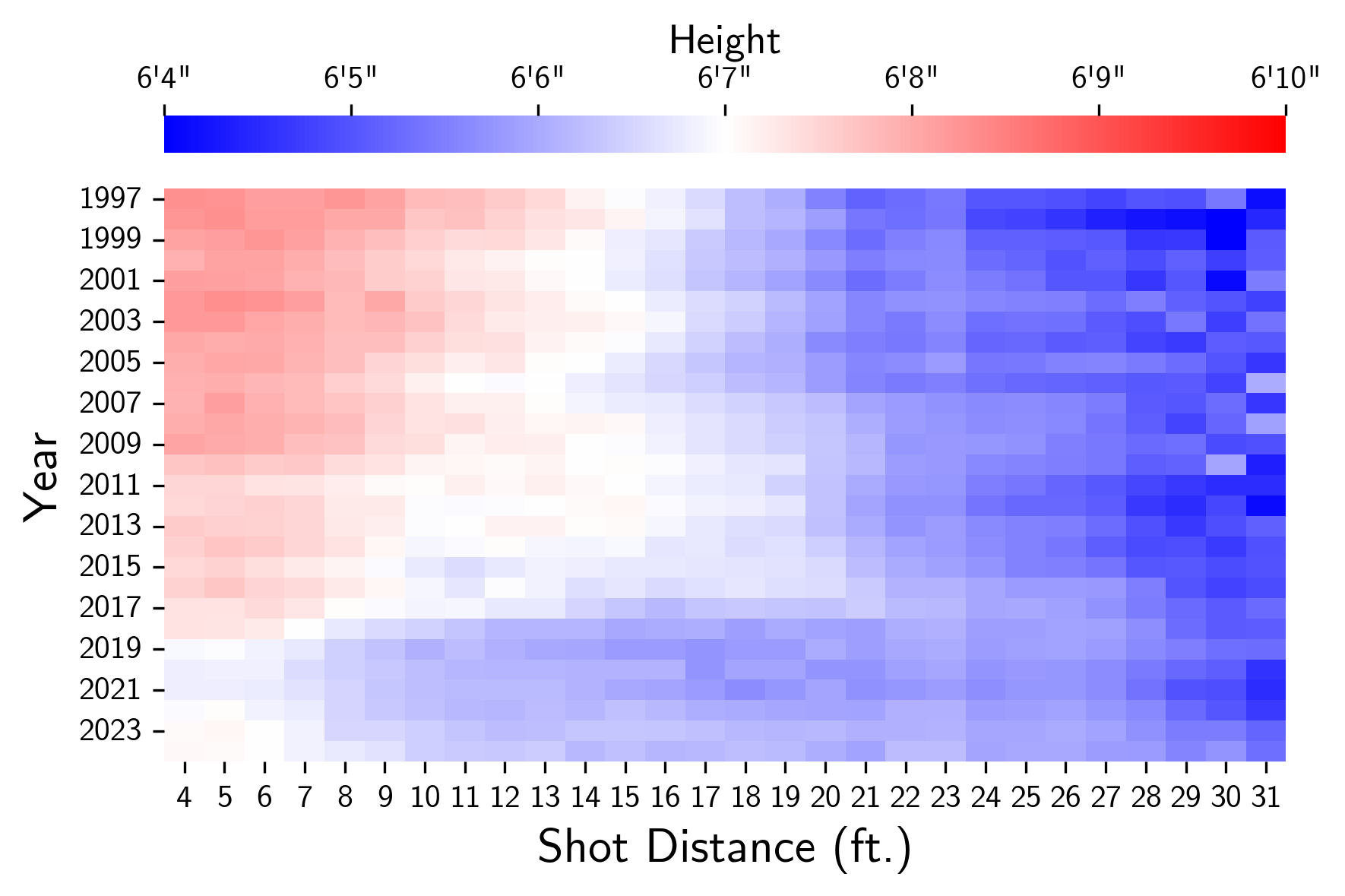
Another way to visualize this trend is through the average shot distance over time, shown in the bottom right panel. From 1999 to 2019, the average shot distance increased by 3 feet, which one might be tempted to attribute to the substitution of deep twos (~22 footers) for threes (~25 footer). But it’s not that simple, and I think the sharp dip in average shot distance around 2010 highlights this. Shot distance is much more granular than jump shot zone distribution and better captures the slow change in basketball philosophy that occured during the past two decades.

Jump Shot Attempts by Distance

My first thought was that the dip in average shot distance could be result of the embrace of the corner three. Maybe teams and players were beginning to acknowledge that 3>2, but were not yet ready to accept that if you practice enough, you can shoot a high volume of 25 footers at a reasonable clip. The corner three would be like the gateway drug, its a closer shot than an above the break three, but still takes full advtange of the fact that more points is better.

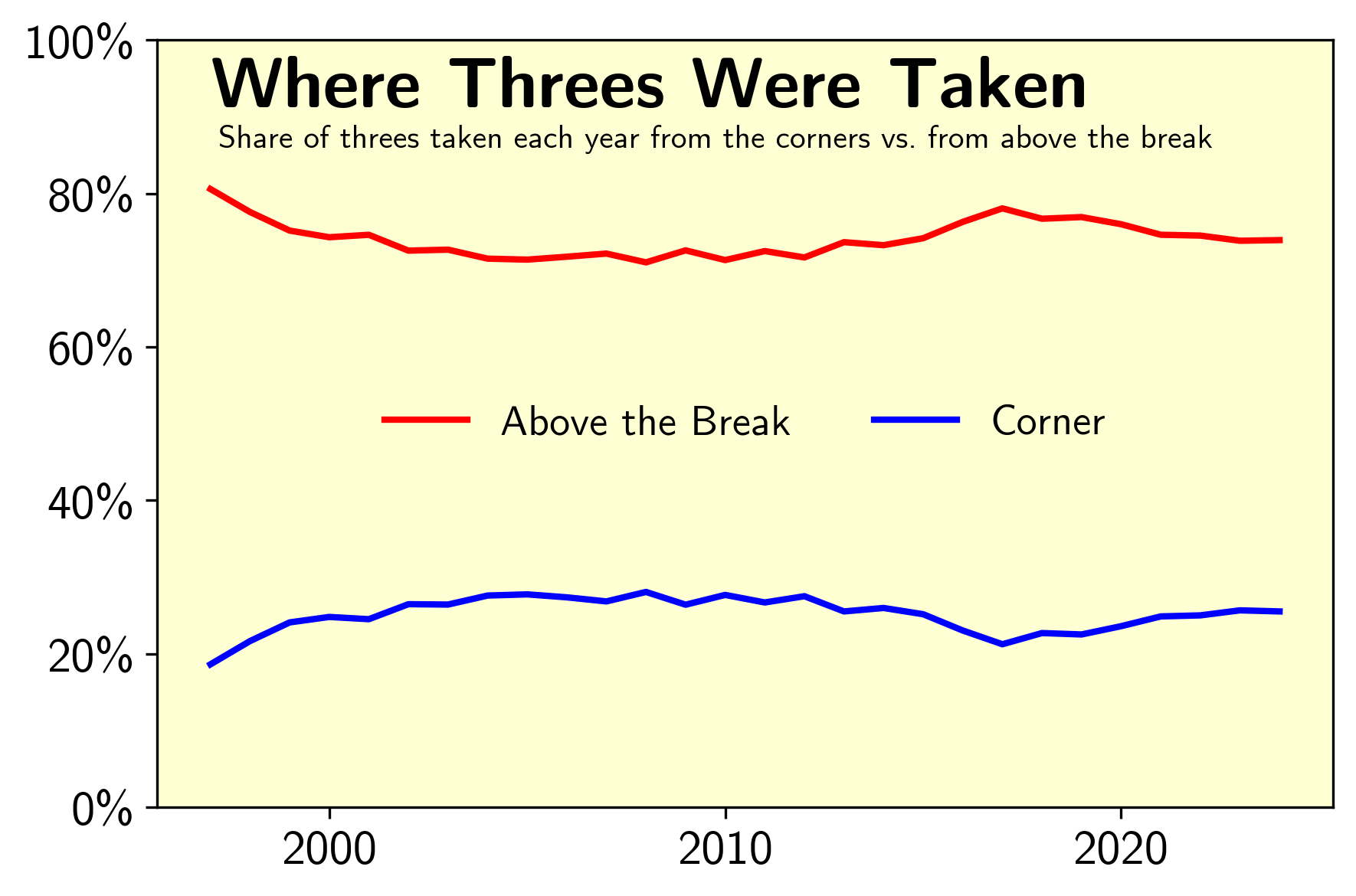
This was not borne out in the data. While distribution of threes showed a small tilt towards corner shots, this trend plateaued by the mid-2000’s. In fact, there is actually a dip in the share of threes shot from the corners around 2016, which is right around the time when “deep three’s” entered the playbook.

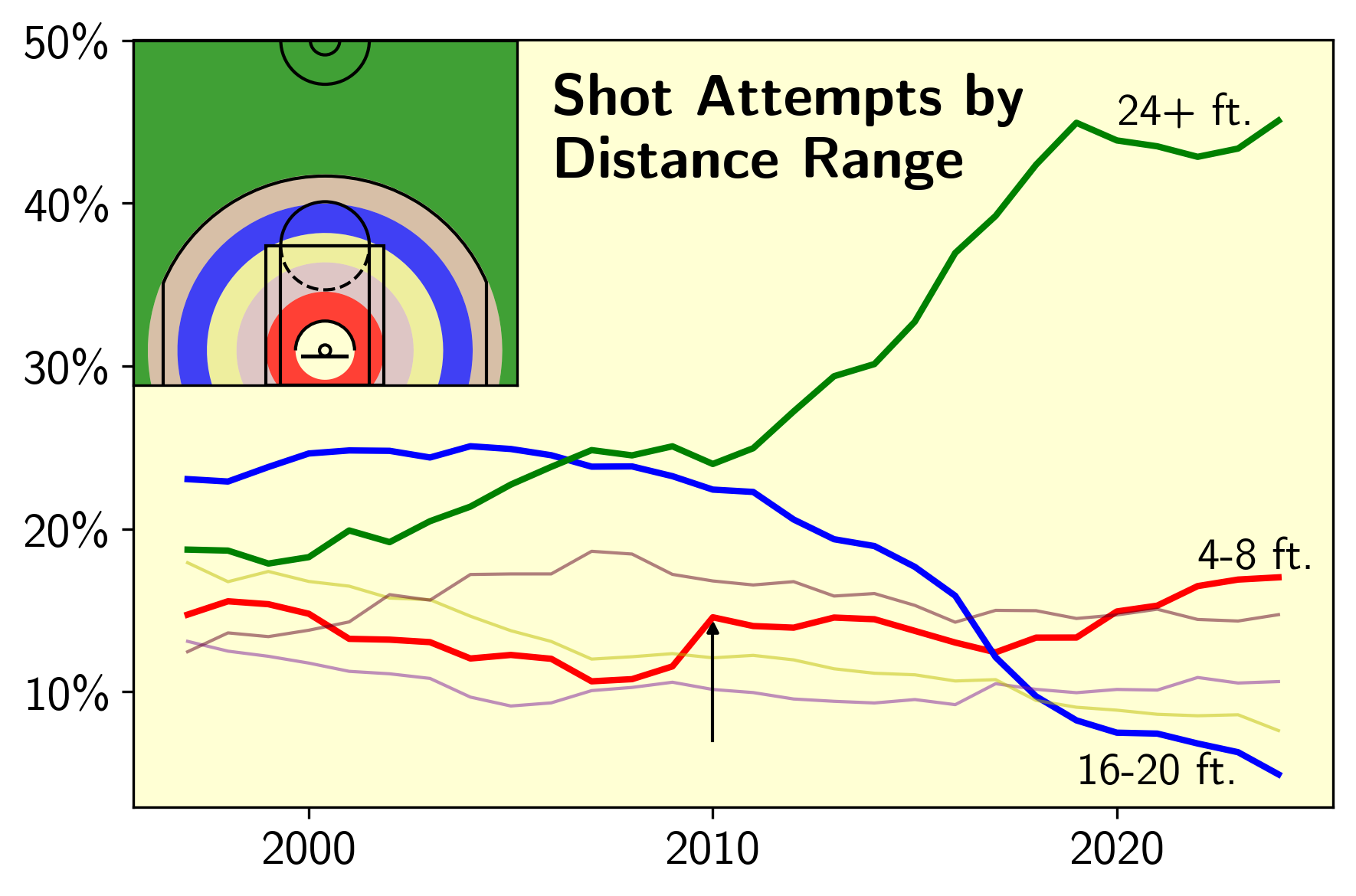
I then broke down the yearly distrubition of shot attempts by distance, splitting into 4 foot ranges (4-8 ft., 8-12 ft., etc.). These ranges are depicted in the upper left inset of the above plot. The dip in the average shot distance around 2010 can be attributed to a decrease in the number of deep two’s taken (blue, 16-20 ft.), coupled with an increase in the number shots near the rim (red, 4-8 ft.) and a relative plateau in the number of threes attempted (green, 24+ ft.). So it seems that the mid range was on its decline, but the three point revolution had not yet fully commenced.

I think that this embrace of the paint jumper can more or less be tied to the decline of the big man. Looking at the top shot attempters in this distance range by year, the 90’s and early 00’s were dominated by bigs (Shaq and Duncan), but by 2010, we start to see more big guards and forwards (Kobe and Shawn Marion crop up in the top 5). In this current area, the list of top shooters in the 4-8 ft. range is filled with big guards, like Harden, Luka, Cade Cunningham, and Josh Giddey. As the paint got less clogged, more shots opened up close to the basket, and players started to take advantage.

I look foward to playing around more with this dataset and the others accessible using nba-sql!

nba_api

The first task was to get familiar with the nba-sql library. This library draws quite a lot from the popular nba_api Python library, which I have used for simple queries over the years. Both use the Python requests package to scrape the NBA’s stats webpages for data (from “endpoints” - undocumented locations within stats.nba.com containing undocumented sets of data), but nba_api simply returns the results of these queries as pandas DataFrames. This is really only helpful for lightweight data analysis, highlighting the main purpose of nba_api:

A significant purpose of this package is to continuously map and analyze as many endpoints on NBA.com as possible. The documentation and analysis of the endpoints and parameters in this package are some of the most extensive information available. At the same time, NBA.com does not provide information regarding new, changed, or removed endpoints.

nba-sql

The nba-sql library allows you to scrape data from ten different endpoints:

• player_season
• player_game_log
• play_by_play
• play_by_playv3
• pgtt
• shot_chart_detail
• game
• event_message_type
• team
• player

In all cases, the general framework of collecting the data is the same:

• Determine a set of parameters for the query (e.g. a list of game id’s number for player_game_log or a collection of (player id, team id, season) trios for short_chart_detail).
• Use the requests package to get the data contained in the endpoint. The previously determined parameters, along with some predefined defaults, are fed into the get function, which essentially tacks them on in a specific way to the end of stats.nba.com/stats/{endpoint}/ before accessing the webpage. A “header” is also passed along in the request, which is a list of settings that are used to trick stats.nba.com into thinking that the site is being visited by a human using a browser, rather than a data-scraping bot. My understanding is that many websites that host data are okay with scraping, as long as some guidelines are met (minimum time between requests, for example). But if you aren’t careful, yor IP address can be blocked from accessing a site (this has happened to me with baseball-reference many times…).
• The data is generally stored in some type of table. After identifying the columns of interest (this is where nba_api comes in), the desired values from each row in the table are stored in an array.
• This array (list of data rows) is then populated into an SQLite database nba_sql.db. This is done using the python library peewee. This is my first experience using an ORM - in my previous data scraping projects, the datasets were either small or the data structures were simple enough to use flat CSV files. An ORM allows you to use Python object oriented programing principles to create, insert data into, and modify SQL databases. This is particularly useful for relationship databases, where the rows of the various tables are related to each other using keys (player id, team id, and game id being examples). In nba-sql a selection of tables (peewee Model objects), corresponding to stats.nba.com endpoints, have been defined with their corresponding fields. During the populate stage, the data is inserted into these tables (models), which are bound to a local nba_sql.db database file. This file can then be queried as pleased.

\[\tilde{}\]