NBA Matchup Predictor
Predicting the result of a matchup in any sport is a challenge. Sportsbooks use sophisticated models trained on large quantities of historic data that are frequently updated in real time information like consider injury reports and market behavior. But setting a money line or point spread essentially boils down to a data science problem, and with access to nearly 30 years of NBA data, one that I can try to tackle.
The goal of this project is to explore the ability of different ML models to predict the outcome of NBA game based solely on data from each team’s games played before the matchup. I’ll explore various aspects of feature engineering, compare models of varying complexity, and attempt to distill the key factors that can swing a matchup. But before we start, we must establish baselines to compare our models against.
Some Notes About the Dataset
- Each season from contains \(\left(82 \times 30\right)/2\) ~ 1,200 matchups, which are stored are as ~2,400 total games (one row for each team in each game).
- There are 28 total seasons in the dataset, spanning 1997-98 to 2024-25. Of these 28, I have omitted four:
- The two lockout seasons, 1998-99 and 2011-12
- The two seasons most affected by COVID, 2019-20 and 2020-21
Bayes Rate
After defining a ML task, one must determine the best possible performance they should expect to achieve with their model. This expert level performance is what is called the Bayes rate in the context of Bayesian statistics and can be thought of as the inherent uncertainty baked into the problem. For the task of predicting NBA matchups, a sportsbook’s money line can act as the expert’s prediction — their models are sure to be stronger than ours, so they should provide a good benchmark.
Historic betting data is more difficult to scrape from the web than the stats provided by stats.nba.com. Many of site that host this data keep it behind paywalls, and the open data that is available is not exhaustive. Thankfully, a kind patron of one of these subscription-based sites published their betting history data on Kaggle for public use. It was stored in a single, flat CSV, and didn’t contain many of the columns used as primary keys in my SQL database, but after some wrangling and cleaning, I was able to insert this dataset into my database for use in this project.
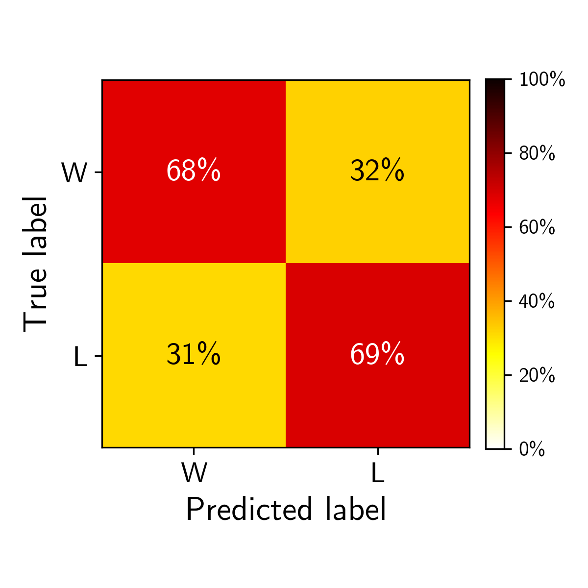
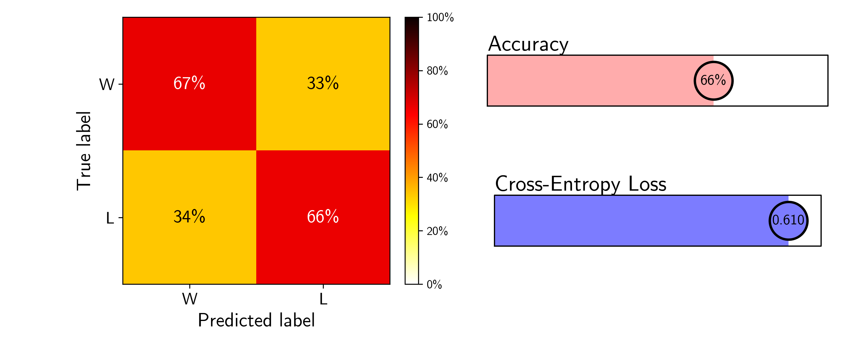
Since the 2007-08 season, the earliest the betting history dataset going back to, the team favored by the sportsbooks (i.e. the team with a negative spread) has won 68.7% of games. This defines our Bayes rate — if my model can predict wins with an accuracy above 68.7%, I will deem this project a success. A confusion matrix provides a nice visual for how the sportsbooks’ predictions perform for each class (wins and losses).
Simplest Win Projector — Home Team
It is also helpful to define a minimum performance baseline that we are sure our model will perform better than. A simple one would rely only on home court advantage — without knowing any details about a matchup, it’s not a bad guess to predict that the home team will win. And this is borne out in our dataset: across the ~40,000 total regular season matchups, the home team won 58.8% of the time. We can use this to inform our lower baseline model and define a Bayesian prior — before considering any team specific data, what is the likelihood of observing a win given our real-world, historical knowledge of the NBA. Our simple model will simply predict
\[P(\text{A beats B}) = \begin{cases} 0.588 & \text{if A is home team} \\ 1-0.588 = 0.411 & \text{if B is home team} \end{cases}\]and assign a win to the home team every single time.
Since our models predict win probabilities, not just W/L, to score our them we will use three metrics:
- Accuracy score (i.e. # correct predictions / # total predictions)
- Cross-entropy loss (i.e. negative log-likelihood)
- Confusion Matrix (i.e. breakdown of true/false positives/negatives)
Since our dataset is perfectly balanced between the two classes of outcomes, the accuracy score provides a simple and descriptive way to evaluate how well our model is at performing the task at hand (predicting matchups). The cross-entropy loss is a gauge of how well-calibrated our classifier is, penalizing confident wrong predictions, and providing better feedback for a model that predicts the probability of an event occurring. And finally, the confusion matrix shown, as shown above. Since our data has exactly as many true wins as true losses, we should expect similar behavior within each true outcome.
Our three metrics for this simple model are displayed below.
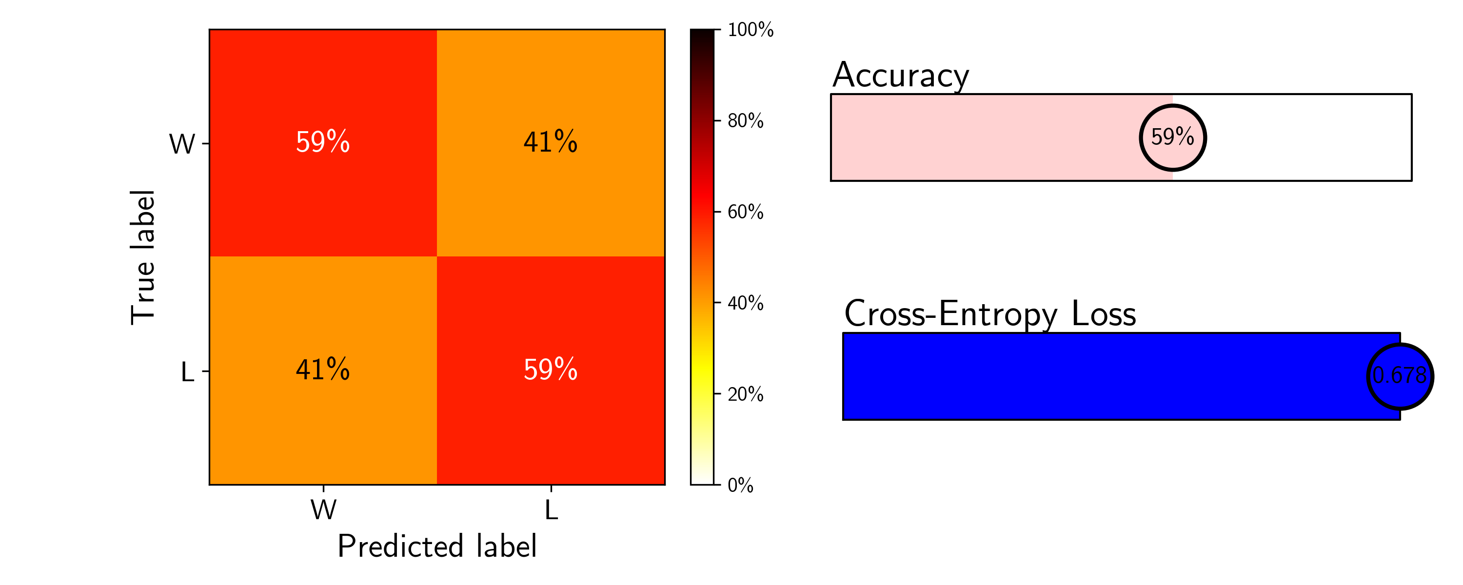
The accuracy of this model is 59%, as expected, and because it predicts a flat win probability, it performs identically across both wins and losses. The loss is large though, relatively speaking — a completely uninformed model that predicts wins and losses with a constant probability of 50% has a cross-entropy loss of ~0.693. To provide a scale to compare the loss for our future models, we will use the value from this baseline model as the max loss we aim to improve upon. We can now begin to provide our model with team context.
Season-to-Date Win%
A simple step up from our baseline model is to predict matchups based purely on team win % at the time of game. If Team A has a higher win % than Team B, then our model will predict that Team A will win the matchup, and vice versa. A softer model may instead produce the probability that Team A/B wins, using the simple Bradley-Terry (BT) model:
\[P(\text{A beats B}) = \frac{\text{W}\%_{\rm A}}{\text{W}\%_{\rm A} + \text{W}\%_{\rm B}},\]where our classifier would then assign a win to Team A if \(P(\text{A beats B}) > 0.5\). We expect that a teams season-to-date win percentage will need time to stabilize, so I will predict matchups only after each team has played 10 games (chosen somewhat arbitrarily here, but explored in more detail below).
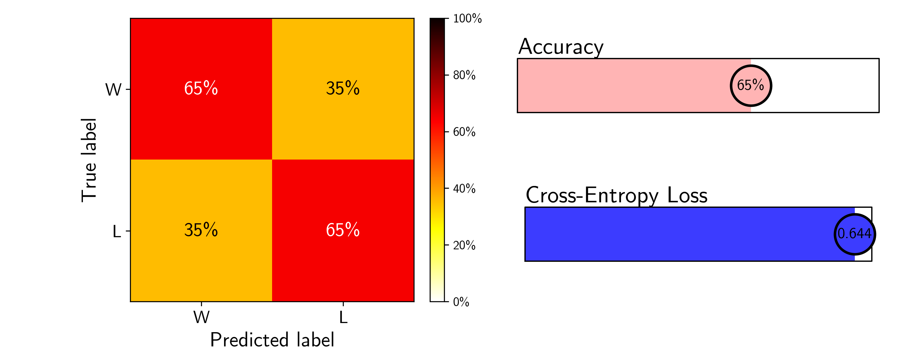
This simple win model has an overall accuracy of 65%, already not so bad. The loss has been reduced slightly but can certainly be improved further with stronger feature engineering and a more complex model architecture.
Four Factor - Running Average
Dean Oliver, one of the pioneers of basketball analytics, developed the “four factors” as a simple and powerful method to predict basketball success. The four factors aim to isolate the most impactful contributors to winning: shooting, turnovers, rebounding, and free throws. They can be broken down into eight stats, four for offense and four for defense:
- Effective Field Goal Percentage
- Turnover Percentage
- Offensive Rebound Percentage
- Free Throw Rate
- Opponent’s Effective Field Goal Percentage
- Opponent’s Turnover Percentage
- Defensive Rebound Percentage
- Opponent’s Free Throw Rate
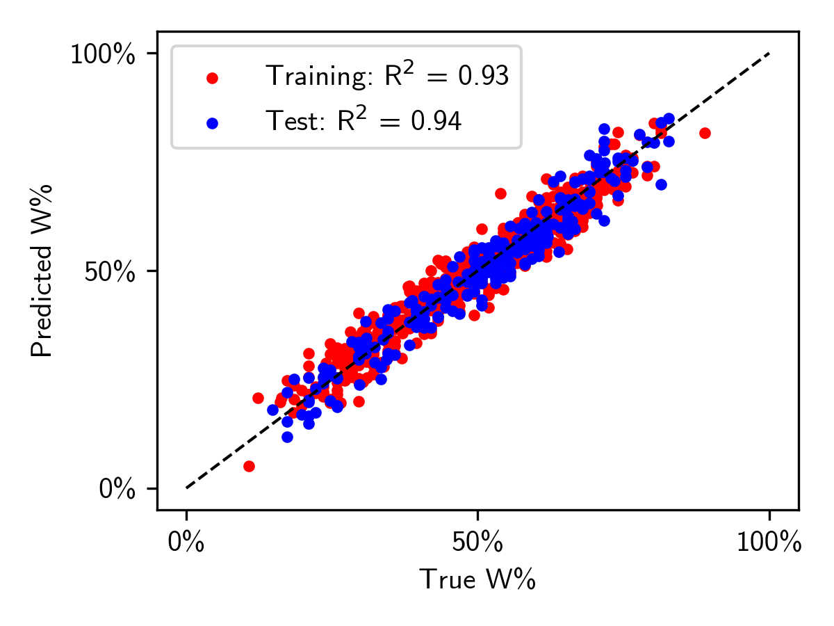
It’s well known that NBA team performance in these eight statistics correlates very well with end of season win percentage. Our linear regression confirms this, with all features exhibiting high statistical significance (\(p \ll 0.05\)). This begs the question, do these stats hold the same predictive power on a game-by-game basis?
To test this, I used the team box score data scraped stats.nba.com of (see my post on the evolution of the NBA shot chart for details on this process). This data set has all the information I need to calculate the rolling average four factor statistics at any point in a season for any time; these will be the features I use in a generalized linear model (i.e. logistic regression model) to predict matchup outcomes. The feature matrix is illustrated below:
| Matchup | Team A Four Factors (Off.) | Team A Four Factors (Def.) | Team B Four Factors (Off.) | Team B Four Factors (Def.) | Context |
|---|---|---|---|---|---|
| \(A_1\) vs. \(B_1\) | ▇▁▅▃ | ▆▂▃▅ | ▇▆▃▁ | ▄▂█▁ | ▄▂█▁ |
| \(A_2\) vs. \(B_2\) | ▃▆▁▇ | ▄▁▆▃ | ▅▁▄▇ | ▂▇▃▁ | ▄▂█▁ |
| … | … | … | … | … | … |
| \(A_N\) vs. \(B_N\) | ▃▆▁▇ | ▄▁▆▃ | ▅▁▄▇ | ▂▇▃▁ | ▄▂█▁ |
Each row represents a single matchup, and the columns correspond to the 2 \(\times\) 8 four factor stats for each team, averaged over all games within the season leading up to the matchup. I also add some “context” stats that I expect will help inform the W/L decision: season-to-date win percentage for each team, as used in the previous model, whether Team A or B is at home (one-hot encoded), and how many days of rest both Team A and Team B have. In total, there were ~40,000 rows of data.
Generating this feature matrix required some simple processing of the basic box score stats, a self-join on game_id with a filter to remove duplicates (to calculate the defensive four factors), a running average aggregation to generate season-to-date statistics, and another self-join on game_id to combine the aggregated data for both teams in each matchup. The initial query of the box score data was done using SQL, but much of the heavy lifting was done in Python, using pandas.
Here are the results of the trained logistic regression model on the test data (75%/25% split). Again, all features were statistically significant (\(p \ll 0.05\)).
While the accuracy improved only modestly, the cross-entropy loss has reduced more substantially, indicating that this model predicts wins and losses more confidently than the simple win percentage-based BT model. It is interesting to note that the form of the BT model can be simply related to the sigmoid function used to generate probabilities in logistic regression, if team strength is instead reparametrized as an exponential. In this case, team win percentage is not the most appropriate metric to use, and something like the ELO rating common in chess would be better. Calculating ELO rating for NBA teams would be an interesting extension to this simple BT model.
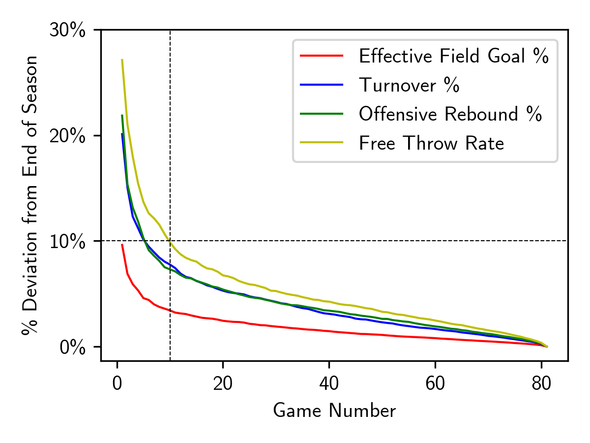
Just as with win percentage model, I imposed the constraint that each team must have played at lease 10 games to be part of the data set, to give some time for the four factor stats to stabilize. Empirically, it appears that the four factor stats stabilize at different rates (see plot on left). But after around 10 games, on average, each stat is within 10% of its end of season value, implying some level of stabilization. Choosing a larger cut off could improve the model, but at the cost of being able to predict fewer outcomes within a given season. We can explore this balance using cross-validation.
Choosing a Minimum Games Played Cutoff
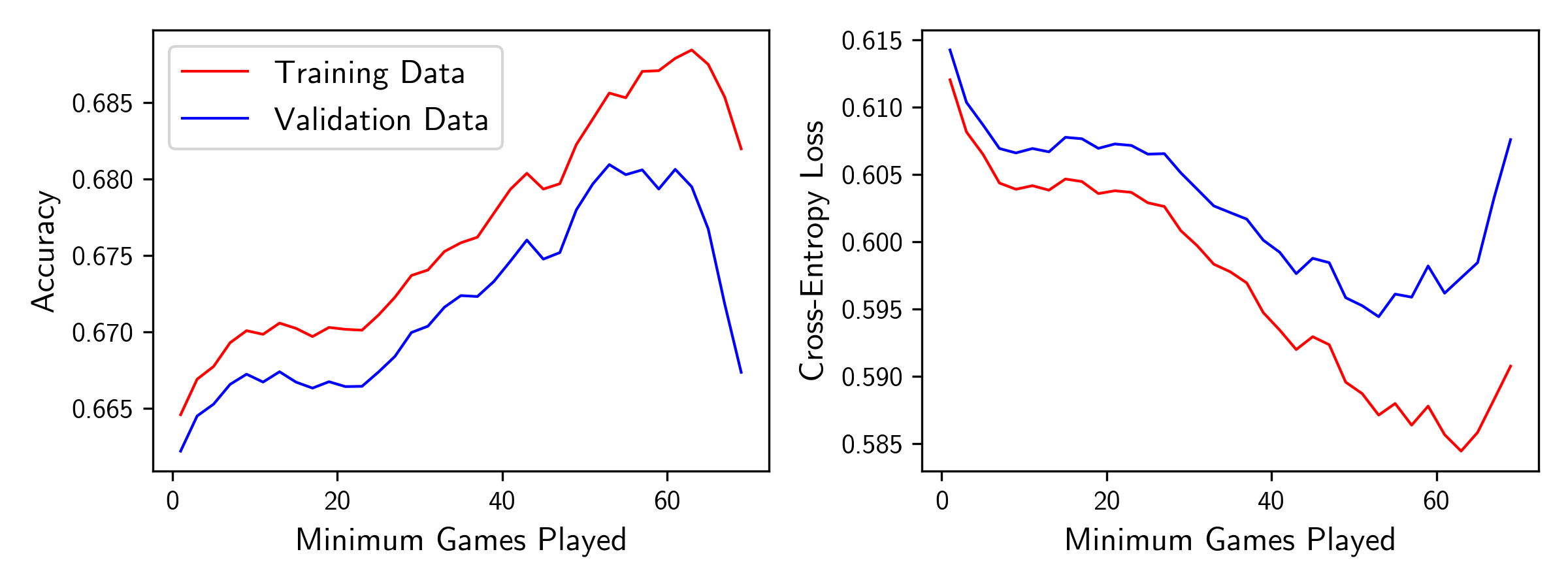
Two choose an optimal minimum game cut off, I further split the training data into a smaller training set and validation set (75%/25% split, once again). I trained the model on subsets of the training data set, pruning to keep only matchups where both teams played a set minimum number of games, and evaluated the result on the validation data. After 60 repeats, I plotted the average training/validation accuracy and loss versus the minimum game cut off used, shown above.
The running average stats for each team become more robust as the cut off increases, which results in an improvement in the model’s performance on both the training and validation data sets. However, at a certain point, the training data size becomes too small, and the predictive power of the model starts to deteriorate, resulting in poorer performance on the validation data.
It’s interesting that the performance on the training data seems to somewhat plateau between the 10 and 30 game cut offs. Perhaps this suggests that there are two stages of stabilization: there is a lot of early season variation that flattens out quickly, followed by more long-term stabilization, perhaps related to lineup adjustment and trades. This seems challenging to capture with our model and would likely require more sophisticated time series modeling to account for.
In any case, just as our validation results predicts, the model trained using a 50 game cut off indeed performs best on the test data.
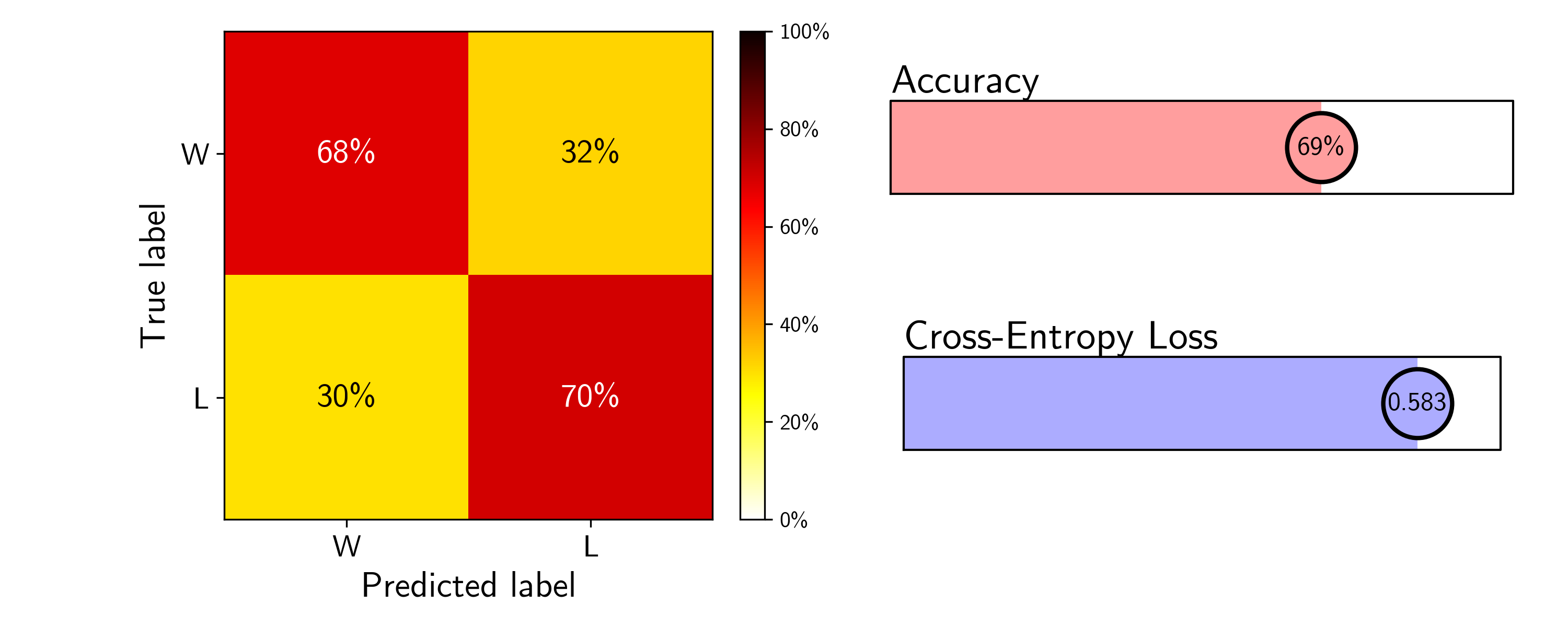
While the accuracy score matches our Bayes’ rate of ~69%, I’m not sure that imposing a 50 game cut off model really represents an improved model. The lower loss implies that the predictions are better calibrated, but only being able to predict games 51 through 82, as opposed to 11 through 82, is fairly constraining for only a 3% increase in the model accuracy from the 10 game cut off model. And since the sportsbooks’ predictions don’t require such a cut off, I’m hesitant to say this model matches their performance. To reach
Future Directions
I had planned to explore the use of models more complex than logistic regression. Logistic regression is at its core a linear model, and it’s unlikely that wins and losses can be neatly separated by a linear decision boundary in our feature space. I trained a variety of different models to address this:
- Random Forest Classifier
- Gradient Boosted Trees
- Support Vector Machine with various kernels
- Dense Neural Network with 1, 2, and 3 layers
None of these models provided a noticeable advantage. My initial thought process was that there are nonlinear relationships between these features, and perhaps these more complex models can capture them. But this highlights the concept of a Bayes rate — if the experts can’t disentangle these relationships, the task is likely just too difficult.
Another possibility is that I’m missing some important latent variables. You can only extract the signal that is in the dataset, so if I’m missing some key pieces of this signal, my model is sure to underperform. Some potential features that can be added:
- Injuries – Perhaps in the form of minutes per game lost due to injury.
- Strategy or roster changes — Adding the rolling average four factor stats over 5, 10, or 20 game windows would be a way to incorporate this temporal information.
- Individual matchup dynamics — One of the most important factors in a matchup is how the two play styles of the team’s fare against each other, but this information is difficult to both extract and encode numerically.
I have already experimented with including rolling averages along as features and incorporating injury information, but more exploration is needed. Another future direction would be to granularize the model in some way. A tanking team and a team pushing for a playoff spot will approach a matchup very differently, and this could perhaps be captured by a hierarchical model.
Conclusions
As a final note on this project, I want to compare the makeup of the incorrect and correct predictions made by my model and by Las Vegas. I will do so using a crude metric: the average magnitude of the spread. A matchup with a large absolute value of the spread represents a matchup where one team is heavily favored over the other, and both models should perform well. A spread close to zero corresponds to a tossup, and I expect both models to perform poorly. The results on the test data are shown in the table below (3,442 matchups):
As expected, the average magnitude of the spread is much closer to zero when the models disagree, 2.9, since this denotes that the classification problem is more difficult. I don’t think much can be taken from the difference in the average spread magnitude when my model is correct/Vegas is wrong and vice versa — this difference of 0.6 is small in comparison to the distributions of spreads within each group. But what’s more notable is the relatively larger average spread when both models are incorrect, 5.3. This suggests that the models aren’t misclassifying purely because the matchup is a tossup, but instead there are some important variables not being considered by both my model and the sportsbooks. With stronger feature engineering, I hope to be able to distill what exactly these variables are.
| Fraction | Average |Spread| | |
|---|---|---|
| Model only correct | 5.6% | 2.6 |
| Vegas only correct | 6.9% | 3.2 |
| Both correct | 61.9% | 7.4 |
| Neither correct | 25.6% | 5.3 |
| Model & Vegas Agree | 87.5% | 6.8 |
| Model & Vegas Disagree | 12.5% | 2.9 |